Walkthrough Example
This is a basic walkthrough of the some of main features of Trips-Viz using an example dataset, for detailed information on each section see the relevant heading further down this page.
Visualising a individual transcript.
From the homepage click on Saccharomyces cerevisiae, then sgd, then Single transcript plot.You will see the page shown in the screenshot below:
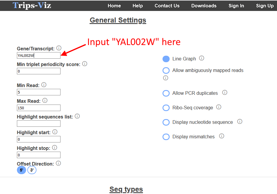
Enter the transcript id "YAL002W" in the Gene/Transcript input box. Leave the other settings at their default values, you can read more about them in the single transcript plot section
further down the page, or by clicking the information icon next to them.
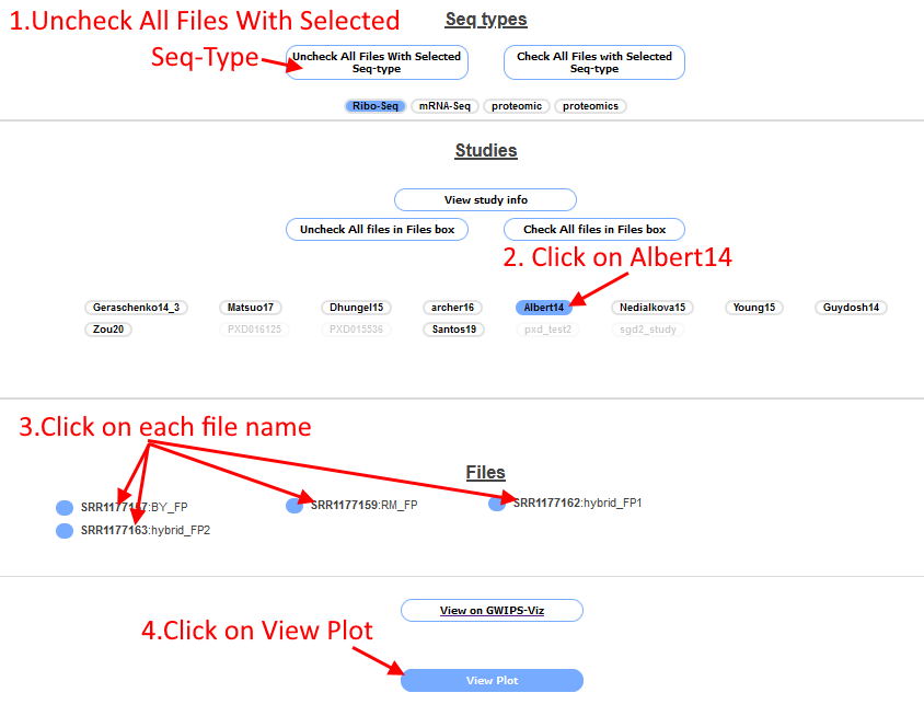
Scroll to the bottom of the page and click the box "Uncheck All Files with Selected Seq-Type", this will unselect all Ribo-Seq files (which are turned on by default). Then
click on "Albert14", the Ribo-Seq files associated with this study will appear in the "Files box". Select each of the four files by clicking on the file name (the circle next to the file name will
be filled in blue to indicate it is selected). Click the "View plot" button at the bottom of the page.
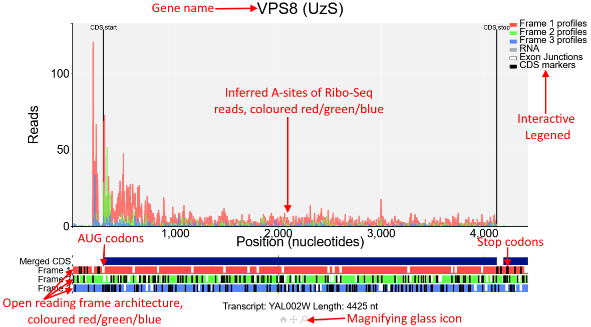
You will see the plot shown in the screenshot above of the gene VPS8 (transcript id YAL002W). In the main part of the plot inferred A-sites of Ribo-Seq reads from the study Albert14 are displayed.
These reads are coloured red/green/blue.These correspond to the open reading frame architecture shown beneath the plot, where each of the three reading frames are represented by a horizontal bar also coloured
red/green/blue. AUG codons are denoted by short white lines, while stop codons are longer black lines.
The annotated CDS start and CDS stop are denoted by vertical black lines on the main plot and
correspond to a start/stop codon in the first reading frame beneath the plot (red). As expected Ribo-Seq reads are mostly contained between the CDS start and CDS stop and biased toward the first
reading frame (red). However there is also a region upstream of the CDS start that also has high Ribo-Seq density and is also biased toward the first reading frame. Click on the magnifying glass beneath the
plot and draw a box around this region to zoom in.
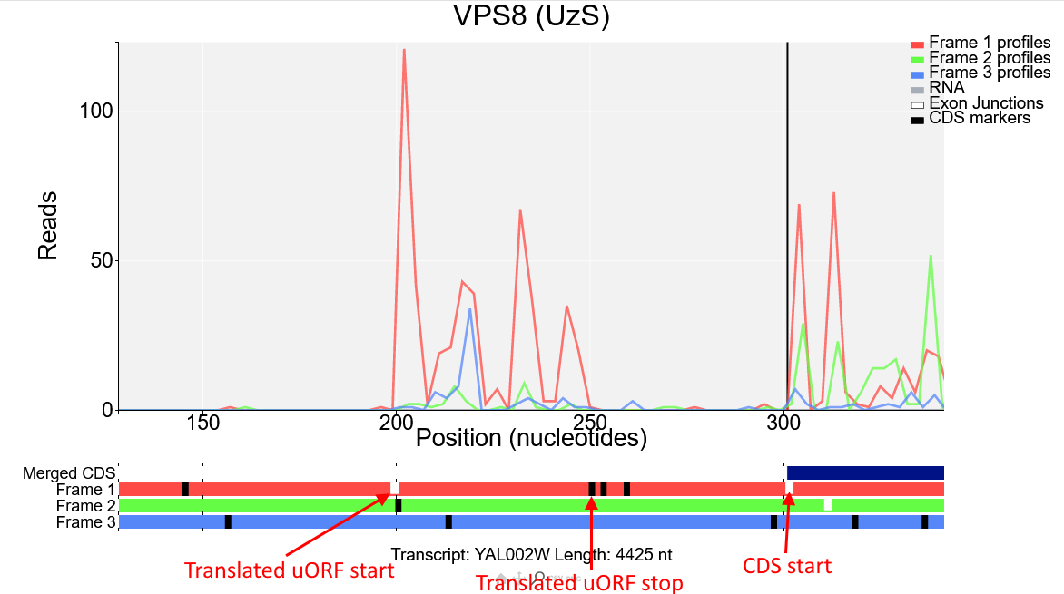
We can see from the reading frames beneath the plot that there is an AUG codon (short white line) right where the read density increases, and a stop codon (longer black line) where the read density drops, this ORF is in the first frame (red) and as the Ribo-Seq reads in this region are also mostly red it is likely that this is the start of a translated upstream open reading frame (uORF) in the first reading frame.
The above can be repeated to view the same gene with data from other studies to see if the uORF is also translated in other studies or is perhaps specific to a certain condition. This can also be done for other genes to find other uORFs or other cases of atypical translation. The single transcript plot page is useful for exploring these specific cases when you have a gene/transcript in mind that you want to explore. If you don't have a specific gene/transcript in mind and are looking specifically for cases of translated uORFs or other ORF types then see the translated ORF detection page.
Detecting translated ORFs.
From the homepage click on Saccharomyces cerevisiae, then sgd, then Translated ORF detection. On that page you will various settings broken into the categories ORF Type, Features and Filters. Leave these settings as default, for detailed information on these see the relevant section further down this page or click on the information icon next to the setting. Scroll down to the sequence types and studies section as on the Single transcript plot page. Click the box "Uncheck All Files with Selected Seq-Type" then click on "Albert14" and select the four Ribo-Seq files as before. Then click the Generate Table button.
After a short while (Note: Wait time will increase when more data is selected, and for organisms with more annotated transcripts) a table will be shown as in the screenshot below:
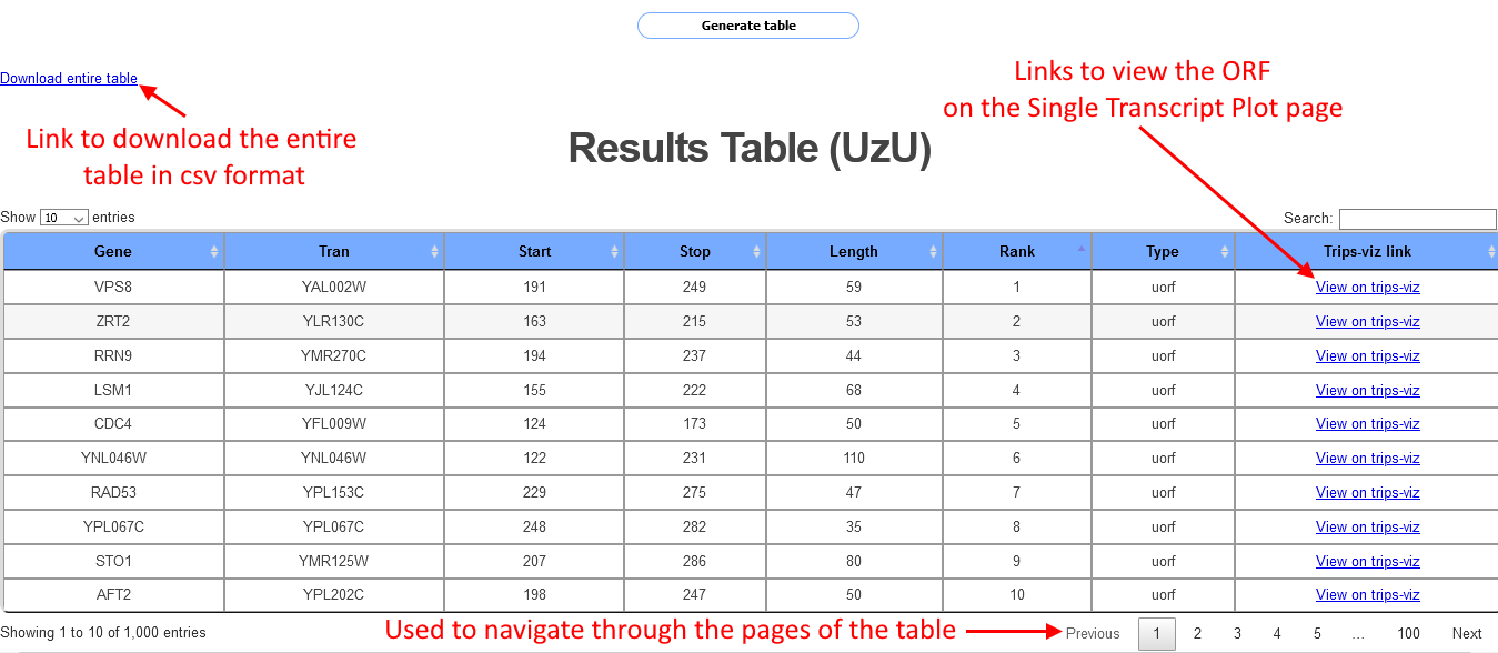
Each row in the table corresponds to a different ORF, information shown for each ORF includes the start and stop position, the length the transcript id and the gene name. Each row also includes a link to the Single transcript plot page. Clicking on the link will open a separate tab where the transcript will be shown with the Albert14 data already loaded and the ORF will be highligted in yellow. Clicking on the arrow on the bottom right of the table will show the next page of the table. This table can show up to 1000 cases of ORFs, in cases where there are more than 1000 cases a csv file with all the cases can be downloaded via a link at the top left of the table.
The above can be repeated for different ORF types which can be selected at the top left of the page as well as using different studies or an aggregate of studies. Note however that ORF detection works best with studies that have strong triplet periodicity. This can be checked on the meta-information page.
Meta-Information.
From the homepage click on Saccharomyces cerevisiae, then sgd, then Meta-Information. At the top left of the page you'll see various different plot types. Click on the triplet
periodicity plot. At the top right of the page is a section for options which will change depending on the chosen plot type. Leave them on default for now. Scroll down and choose the four files from
the Albert14 as before, then click view plot. You'll see the plot shown in the screenshot below:
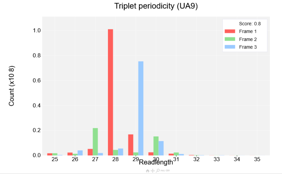
Read lengths are shown on the x-axis while the count is shown on the y-axis. Each read length has three bars corresponding to each of the three reading frames. If a dataset has strong periodicity one of the reading frames will be much higher than the other two. A score is also shown at the top right of the plot between 0 and 1, with 0 being the worst periodicity and 1 being the best. The better the periodicity the easier it will be to detect ORFs and the clearer it will be when visualising single transcripts.
The other plot types at the top left of the page can be used to check other aspects of datasets such as the read length distribution or metagene profiles, which can be useful when assessing a datasets quality. A description of each can be seen in the metainformation section further down this page or by clicking the information icon next to the plot name.
Differential expression/translation
From the homepage click on Saccharomyces cerevisiae, then sgd, then Differential plot. Leave the settings at the top of the page at their defaults. Scroll down and click on Albert14.
The file selection works a little bit differently for this page than the previous ones.
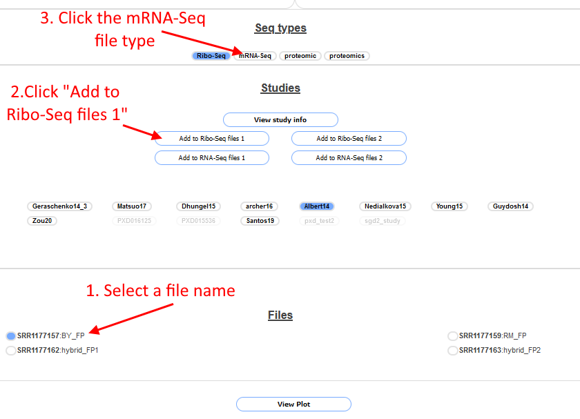
Only one file can be selected at a time. First click on the file SRR1177157 to select it (1. In screenshot above), the circle will turn blue to indicate which file is selected. Next click on "Add to Ribo-Seq Files 1" (2. In screenshot above), then click
on the file SRR1177159 to select that and again click "Add to Ribo-Seq Files 1". Next do the same for SRR1177162 and SRR1177163 but click the "Add to Ribo-Seq Files 2" button instead. Then click on the mRNA-Seq button in the
Seq-Types section (3. In screenshot above), the files in the file box will change. Select the files SRR1177156 and SRR1177158 and press the "Add to RNA-Seq files 1" button after each, do the same for SRR1177160 and SRR1177161 but click the
"Add to RNA-Seq files 2" button after each. When finished scroll up the page, the four boxes should look like the follwing screenshot:
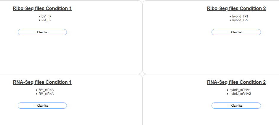
Then click the View Plot button at the bottom of the page. You should see a plot like the following:
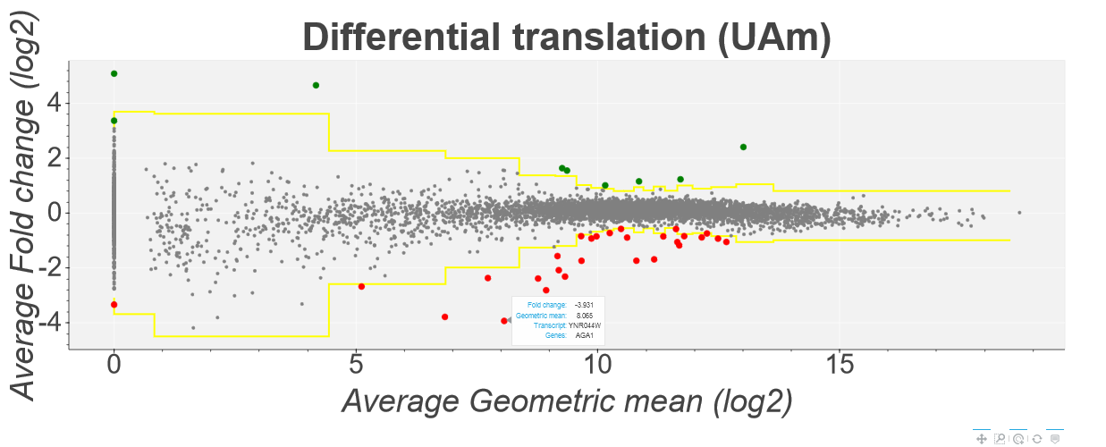
This plot shows the translation efficiency fold changes of each gene in Saccharomyces cerevisiae in the Albert14 study as calculated by the Z-score method. Average fold change is
shown on the y-axis while the geometric mean of the 8 datasets is shown on the x-axis. Points above and below the yellow line represent genes with a z-score higher/lower than 4 (this can be changed using
the inputs at the top of the page). Howevering over a specific point tells you the gene/transcript id of the point as well as the specific fold change and geometric mean. Clicking on a point will open a
seprate tab showing a comparison plot of the Ribo-Seq and mRNA-Seq for each condition. For example:
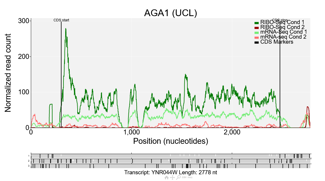
This is a comparison plot for the gene AGA1 showing the data from the Albert14 study. Ribo-Seq reads are shown in dark green/red corresponding to condition 1/2, while mRNA-Seq reads are shown in light green/red corresponding to condition 1/2. The Ribo-Seq reads in condition 1 are much higher than the RNA-Seq reads in condition 1, but for condition 2 the Ribo-Seq reads are lower, meaning the translation efficiency is lower in condition 2 than condition 1. Comparison plots such as this can also be generated manually by going to the comparison plot page directly. Any number of conditions can be plotted there which makes it useful for looking at variation between replicates or comparing more than two conditions.
General Information/Frequently Asked Questions
Why is it called Trips-viz?
Trips-viz is a (poor) acronym standing for TRanscriptome wide Information on Protein Synthesis VIZualized. This is mainly to match the naming of our sister site gwips-viz which provides Genome Wide Information on Protein Synthesis.
Do I need an account to use Trips-viz?
No. All features of Trips-viz can be used without an account. An account is only needed if you wish to change specific aspects of plots such as the background colour. An account is also needed to upload your own data, or to view private data uploaded by someone else.
What are the codes that appear in the titles of Trips-Viz plots?
These are unique codes that are generated for every plot on Trips-Viz. These allow for quickly sharing plots and record the specific files/studies used to generate the plot as well as any settings that were
changed. By following a link in the form https://trips.ucc.ie/short/
How do I share plots?
Can I upload my own data?
Yes. To upload you need an account, then visit the upload link at the top of the page. This is split into 3 sections called "Upload new file", "My studies"
and "My files". The "Upload new file" section allows you to choose an organism, an assembly, a study name, and a sequence type. Once those are chosen you can click the
"Browse" button to choose a file to upload and then press the "Submit" button to upload the file. After the file has been uploaded you'll see the study appear in the
"My studies" section, where the organism, study name and assembly will be listed. There will also be a text box referred to as "Access list" where you can give other
Trips-Viz users access to your data. To do this, enter a list of usernames in the text box and press the "Update" button at the bottom of the page.
The "My files" section will also be populated after uploading a file. This will list the file name, the study name and a checkbox for each file. To delete files click the
checkboxes of the files you want to delete and press the "Delete files" button at the bottom of the page.
Note that any files uploaded to Trips-Viz need to be in a specific format (sqlite) and have the extension .sqlite. In order to create a file in that format, our reccommendation
is to use RiboGalaxy, under the Trips-Viz section select the bam to sqlite tool. Note that this tool requires an annotation sqlite file which
can also be created on RiboGalaxy using the create new organism tool, or downloaded from the Trips-Viz downloads page if the organism is already available there.
Alternatively you can use the "bam_to_sqlite.py" script, which can be retrieved from the downloads page. You will also need to download a file called "transcriptomic_to_genomic.sqlite" and
"organism_name.sqlite" which can be downloaded from the same page. Then run the python 2 script as follows:
python bam_to_sqlite.py
How is the Ribo-Seq/mRNA-Seq data processed?
Publicly available Ribo-Seq/mRNA-Seq data is downloaded from the ncbi sequence read archive. After which it is converted to fastq format and adapter is removed using cutadapt. Reads below 25 nucleotides in length after adapter removal are discarded. Reads are alinged to rRNA sequences using bowtie. Reads that map to rRNA are discarded while remaining reads are aligned to the transcriptome using bowtie. The resulting BAM file is parsed with a python script. Each mapped read is checked to see how many genomic positions it maps to, if only one the read is classed as unambiguous, if more than one it is classed as ambiguous. An offset is also determined for every read by choosing the highest peak near the start codon using the counts from the metagene profile.
Can I upload sequencing types other than Ribo-Seq/mRNA-seq?
Yes. This can potentially be done with any sequencing data that can be aligned to a transcriptome, but you will need to be somewhat familiar with python.The basic steps involve parsing a text file and placing the information in SQLite format. An example of a python script that can do this is provided on the downlods page which you can view by selecting "Scripts" under the group dropdown box and then "tsv_to_sqlite.py" in the file dropdown box. This can be easily modified to parse a csv file. The output will be in .sqlite format which you can then upload to Trips-Viz.
Can I use a custom transcriptome?
Yes. If you have a transcriptomic fasta file and a gtf file you can upload your own transcriptome to Trips-Viz. This can be done by first downloading the
scripts entitled "create_annotation_sqlite.py" and "create_transcriptomic_to_genomic_sqlite.py" from the downloads page (select the "Scripts" group).
Run the "create_annotation_sqlite.py" script as follows:
python create_annotation_sqlite.py <organism_name> <gtf_file_path> <fasta_file_path> <pseudo_utr_len>
where pseudo_utr_len is an integer which can be used to add a flanking region to all transcripts, which can be useful if UTR's are not annotated, set to
0 if UTR's are already annotated. This will produce a file named <organism_name>.sqlite then run the script "create_transcriptomic_to_genomic_sqlite.py" as follows:
python create_transcriptomic_to_genomic_sqlite.py <gtf_file_path> <pseudo_utr_len>
This will produce a file called "transcriptomic_to_genomic.sqlite" (this is needed for the bam_to_sqlite.py script). To upload your transcriptome go to the
uploads page, select the "Upload new transcriptome" tab. Fill in the required fields and upload the .sqlite file that was prouduced by the create_annotation_sqlite.py script.
A message will come up after a some time indicating a successful upload. Navigating back to the home page should show the newly uploaded organism
(this will only be visible by you), files can then be uploaded for that organism just like any other organism on Trips-Viz.
Previously uploaded transcriptomes can be deleted from the uploads page under the "My transcriptomes" tab.
Note the variables with labels such as "search_term_before_transcript" in the create_annotation_sqlite.py and create_transcriptomic_to_genomic_sqlite.py scripts may need to be
changed. This is because gtf files are not standardised so the scripts need to have the terms that appear immediately before and after the transcript and gene ids in the gtf file.
Here is an example of a line in a gtf file and what the corresponding variables should be set to:
gtf line:
chr1 HAVANA transcript 11869 14409 . + . gene_id "ENSG00000223972.5"; transcript_id "ENST00000456328.2"; gene_type "transcribed_unprocessed_pseudogene"; gene_status "KNOWN"; gene_name "DDX11L1"; transcript_type "processed_transcript"; transcript_status "KNOWN"; transcript_name "DDX11L1-002"; level 2; transcript_support_level "1"; tag "basic"; havana_gene "OTTHUMG00000000961.2"; havana_transcript "OTTHUMT00000362751.1";
variables:
search_term_before_transcript = 'transcript_id "'
search_term_after_transcript = '.'
search_term_before_gene_1 = 'gene_name "'
search_term_after_gene = '";'
Single gene/transcript plot
Video tutorial
Plot description
The purpose of this plot is to allow you to see the ribosome profiling and rnaseq reads that align to an individual gene or transcript.
The ribosome profiling reads will be colour coded according to which frame the a-site is found in. If the triplet periodicity of the reads contributing
to the graph is strong then this plot should give a clear picture of which frame is being translated.
The page is split into three parts, at the top of the page you have general settings. Here you can choose settings like, the maximum triplet periodicity
score for each read, the gene you want to view, the minimum and maximum allowed readlengths and many other settings. To get a more detailed description
on any one of these settings simply click the link next to it labelled "(What's this?)", or you can view the explanations further down this page.
At the middle of the page you can select a sequence type. Then click on
one of the studies in the studies box. This will bring up a list of relavent files associated with that study in the "Files" section below. Next to each
file will be a circle. If the circle is filled in this means that reads from that file will be included in the graph. To turn on or off an individual file
simply click the circle next to the file name or the file name itself. As some studies can have many files associated with them, there are buttons in the
studies box that act as shortcuts.
There are 2 buttons in the "Studies" section to turn on/off all files currently in the "Files" section, and another 2 buttons in the "Seq type" section to turn on/off all files from
the selected sequence type. There is also a button in the studies box to "View study info". When pressed this will bring up a pop up which will display information
relevant to the selected study such as a link to the paper and a link to the raw data.
At the bottom of the page there are two buttons the first is "View on Gwips", which when clicked will display the current gene on Gwips-Viz
(note this only works if you've created a plot in Trips-Viz first) the second is the "View Plot" button which when pressed will display a loading screen for a short while after
which a plot and another button will appear below the "View Plot" button. This new button will be labelled "Direct link to this plot", by right clicking on this button and copying
the link you can send the plot to another person (for more information see
How do I share plots? ).
![]()
The main window for the plot will have a read count on the y-axis and the position in nucleotides along the x-axis. Above the main window will be the name of the gene you
are viewing followed by a short code in brackets (this can be used to re-create the plot your viewing). By default only the ribo-seq data will be shown, which is colour coded
according to the frame it aligns to. Just below the main window the orf architecture for this transcript will be shown. The three frames are colour coded red, green and blue.
Start codons are denoted by short white lines, stop codons are denoted by longer grey lines. To the right of the main window is the interactive legend. Elements in the main
window can be turned on/off by clicking the coloured boxes in the legend. Below the orf architecture lies the tools, clicking on the magnifying glass icon will allow you to draw
a bounding box in the main window to zoom into a specific area. Clicking on the four arrows icon will allow you to click and drag anywhere in the main window to move the data.
Finally clicking on the home icon will allow you to undo any affect of the move/zoom tool and reset the view to it's original settings.
Allow ambiguously mapped reads
Checking this box means that both ambiguously mapped reads and unambiguously mapped reads will be displayed. A read is considered ambiguous if it maps to more than one genomic position.
Line Graph
If this is checked then the data will be displayed, as a line graph instead of as individual peaks. This makes no difference to the actual data displayed it is purely an aestethic choice. However, the line graph is less memory intensive and can result in a smoother experience, especially when zooming.
Highlight sequence list
This text box allows you to input a comma seperated list of nucleotide sequences which will be highligted in the open reading frame architecture of the resulting plot. By default these will appear as short black lines but their colour can be changed in the settings. These can be turned on/off by clicking the "Highlighted sequences" button to the right of the plot. Note: the following IUPAC codes are also recognised: R: A/G Y: C/U S: G/C W: A/U K: G/U M: A/C B: C/G/U D: A/G/U H: A/C/U V: A/C/G N: A/C/G/U
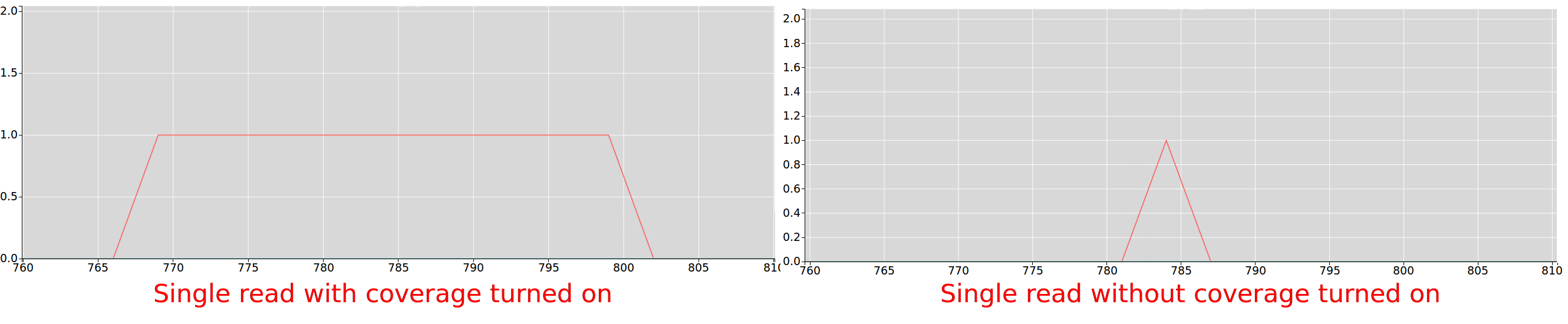
Riboseq coverage
If checked, every position of every read contributes to the data displayed on the plot, if unchecked only the inferred a-site of the read
contributes to the plot.
For more information on how a-site is inferred for trips see.
Max Triplet Periodicity Score
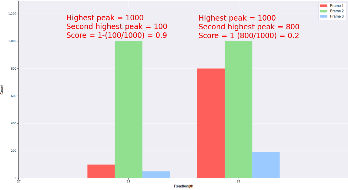
This is a simple metric to include/exclude readlengths from a particular file depending on how good the triplet periodicity is.
For each readlength a score is calculated from it's triplet periodicity plot using the formula 1-(count of the second highest peak/count of the highest peak)
, thus read lengths with very good triplet periodicity will be close to 1, while readlengths with poor triplet periodicity
will be close to 0.
Any readlengths from any files with a read score below what is entered in this field will not be
displayed, thus entering a value close to 1 will result in better triplet periodicity but less data.
Gene/Transcript
The gene or transcript to be plotted. If given a gene with multiple transcripts then a list will be displayed of all transcripts associated with that gene. Transcript ids are based on gencode annotations, refseq will not be recognised.
Min Read
The minimum read length to be displayed on the graph. Any reads below this length will be ignored.
Max Read
The maximum read length to be displayed on the graph. Any reads above this length will be ignored.
Offset Direction
Infer the a-site of each ribosome protected fragment from either the 5' or 3' end of each read.
Nucleotide sequence
If this box is checked the nucleotide sequence of the transcript will be displayed below the main plot. Each nucleotide is coloured according to reading frame, such that the colour of the nucleotide corresponds to the first letter in the codon of the corresponding frame. Depending on the length of the transcript, displaying the nucleotides can add a significant amount of time to the plot generation.
Single gene/transcript comparison plot
Video tutorial
Plot description
The purpose of this plot is to view data from multiple datasets (or groups of datasets) for a single gene simultaneously. This is useful in the case were there are
Ribo-seq datasets generated under treatment and control conditions or as part of a time series and you would like to view what the difference looks like for a
particular gene/transcript.
At the top of the page is the General settings section. This provides the user with options to change the transcript to be plotted, the minimum and maximum readlengths,
or whether to include ambiguously mapped reads. Below General settings lies two boxes, one labelled Studies the other labelled File list. The Studies box contains a
button labelled Add, a coloured square, and a list of studies that have been aligned to the currently selected organism/transcriptome assembly.
Only files listed in the
File list box will be plotted in the graph.
In order to add files to the file list box, a user must click on one of the studies. This will populate the Ribo-Seq files and RNA-Seq files boxes below the Studies box
with a list of files relevant to that study. Clicking on one of these files and then pressing the Add button in the Studies box will place that file into the File list.
As long as the colour in the coloured box remains unchanged, multiple files can be added to the same group in the File list box by continually selecting different files
and pressing the Add button after each selection. If the user does change the colour in the coloured box (a pop up appears when clicking on the coloured box) all
subsequently added files will be added to the File list under the same group.
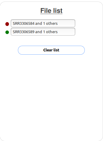
Each group has two files associated with it.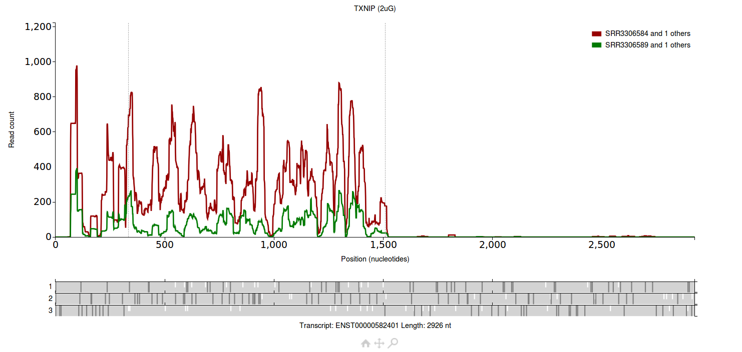
The group plotted in red has two files associated with it (SRR3306583 and SRR3306584), the group plotted in green also has two files associated with it (SRR3306588 and
SRR3306589).
All four files are from Park et al. 2016.
Gene/Transcript
The gene or transcript to be plotted. If giving a gene with multiple transcripts then a list will be displayed of all transcripts associated with that gene. Transcript ids are based on gencode annotations, refseq will not be recognised.
Min Read
The minimum read length to be displayed on the graph. Any reads below this length will be ignored.
Max Read
The maximum read length to be displayed on the graph. Any reads above this length will be ignored.
Highlight start/Highlight stop
These values can be used to highlight a specific region of a transcript. Filling in a value for highlight start and highlight stop will colour in that region of the plot.
Allow ambiguous reads
Checking this box means that both ambiguously mapped reads and unambiguously mapped reads will be displayed. A read is considered ambiguous if it maps to more than one genomic position.
Normalization by mapped reads
When looking at the difference between two groups of files there may be a large difference in the number of mapped reads in each group. Checking this option aims to mitigate the effect of mapped reads differences by determining the factor difference between the groups and then decreasing the counts of the higher groups by that factor. For example if there is one dataset in condition 1 with 1,000,000 mapped reads and one dataset in condition 2 with 500,000 mapped reads, the count for every position in condition 1 would be divided by 2.
Metainformation plots
Video tutorial
Plot description
The purpose of these plots is to allow you to gain insight into specific features of a particular dataset, such as wether or not it has good triplet periodicity.
The top left section of the page allows you to choose a plot type by clicking on it. Some plots have settings that you can change, if these are applicable to this
plot the settings will appear in the options section in the top right of the page.
At the middle of the page is the "Studies" section and "Seq types" section. To choose which files are contributing to the plot, first click on a sequence type and then on on of the
studies in the "Studies" section. This will bring up a list of relavent files in the "Files" section below. Next to each
file will be a circle. If the circle is filled in this means that reads from that file will be included in the graph. To turn on or off an individual file
simply click the circle next to the file name or the file name itself. As some studies can have many files associated with them, there are buttons in the
studies box that act as shortcuts. There are 4 buttons to turn on/off all riboseq/rnaseq files, and another 4 buttons to turn on/off all riboseq/rnaseq files
in the selected study. There is also a button in the studies box to "View study info", when pressed this will bring up a pop up which will display information
relevant to the selected study such as a link to the paper and a link to the raw data. Once you have selected all the relevant files you wish to include in the
plot click the "View Plot" button below the riboseq/rnaseq boxes or press the enter button on your keyboard. The different plots are explained under seperate
headings below.
Readlength distribution
This plot shows different read lengths on the x-axis and their counts on the y-axis. All mapped reads in a file contribute to this plot (wether they map ambiguously or not). This plot can be used to help determine if a file contains genuine riboseq reads or not. In general we would expect the readlength distribution to have a relatively narrow peak centered around ~30 nucleotides for genuine riboseq data.
Nucleotide composition
This plot shows the nucleotide composition across all selected reads in a given range. The minimum and maximum readlengths allowed to contribute to this plot can be controlled in the settings for this plot. Other settings you can change for this plot are the ability to inlcude mapped/unmapped reads. Wether the nucleotides are taken from the 5' end or 3' end of all reads, and wether the absolute counts are shown or percentages at each position. This plot can be used to assess if there is an unusually high number of nucleotides at a certain position in the read. For example if you see a high percentage of A's at the 3' end of unmapped reads it may indicate that polyA tails were not correctly removed from these reads, or a high percentage of T at the first position may indicate a problem with untemplated addition. In frame or out of frame (relative to the CDS) reads can also be selected. Unlike the "All mapped reads" or "All unmapped reads" options these are not precomputed. This means they will take longer to return a plot, it also means any sequence mismatches such as untemplated additions or untrimmed adapter will not be apparent. This may be useful to assess if nuclease bias has an affect on triplet periodicity.
Triplet periodicity
This plot shows the triplet periodicity across a given range of readlengths. The user may decide the minimum and maximum readlengths in the settings for this plot. Each readlength will have three bars associated with it corresponding to one of three frames the reads align to. A particular read length is considered to have strong triplet periodicity if the count in one of the frames is much higher than the other two frames. The legend in the top right will also show a score based on all readlengths in this particular plot. This is done by using the formula: 1-(count of the second highest peak/count of the highest peak), if more than one readlength is shown the highest peaks and second highest peaks of each readlength is summed and then the formula is applied. This will result in readlengths with strong periodicity receiving a score close to 1, while readlengths with weak periodicity receive a score close to 0. The better the triplet periodicity for a given study the clearer it will be which frame is being translated when viewing reads from this dataset on the single transcript plot.
Reads breakdown
This plot shows a breakdown of reads into multiple categories for each file. Categories are as follows
"cutadapt removed": the number of reads removed by cutadapt because they
were too short after trimming.
"rRNA mapped": Number of reads removed because they mapped to ribosomal rRNA.
"Unmapped": Number of reads which could not be mapped to the transcriptome.
"Ambiguous": the number of reads which mapped to more than one genomic location (see "How is the Ribo-Seq/mRNA-Seq data processed?").
"Mapped noncoding": Number of reads
mapped to regions not annotated as coding.
"Mapped coding": Number of reads mapped to annotated coding regions.
The reasons for using this plot would be to assess problems with the mapping, for instance if the majority
of reads were unmapped and the number of reads removed by cutadapt was very low it may indicate a problem with adapter removal. It could also be used to assess wether a file was genuinely
riboseq or not as we would expect a higher proportion of reads to align the the coding than noncoding regions compared to rnaseq data.
Metagene
This plot shows counts on the y-axis and a position relative to some sequence feature on the x-axis, this can be the annotated start or stop codon, or a custom sequence.
All reads from any gene that lie near the chosen position will be plotted, this can be based off the 5' end of reads, 3' end of reads, or the inferred A-site.
Genuine Ribo-Seq data should have a much higher density of reads 3' of the start codon than 5' of the start codon (and vice versa for the stop codon).
The following settings can be changed in this plot:
Include 5' ends/Include 3' ends: Choose which end of the read the counts are based on, only one option can be chosen at a time.
Apply offsets: If checked the offsets used to infer the A-site will be applied to the read counts.
Aggregate: If checked, the counts from all selected files will be grouped together, if unchecked files will be plotted with different colours seperately. A maximum of 6 files can be selected if not aggregating.
Normalise: If checked, counts will be normalised based on the number of mapped reads in each file. This is based on a factor difference between the file with
lowest number of mapped reads and all other files. For example if plotting three files A,B and C which have 100,200,300 mapped reads respectively. The counts
from file A would be unchanged (as it has the lowest number of mapped reads), all counts from file B woudld be multiplied by a factor of 0.5 (100/200 = 0.5) and all counts from File C would be multiplied
by a factor of 0.33 (100/300 = 0.33).
Min/Max readlen: Readlengths outside this range will not contribute to the plot.
Custom sequence list: Rather than centering the plot around annotated start or stop codons multiple custom sequences (seperated via comma) can be entered in this box.
The search limits below restrict where the custom sequences should be searched for, this can be across the whole gene, the 5' leader (5' UTR), the annotated
coding region (CDS) or the 3' trailer (3' UTR). This can be further restricted by the boxes below to include or exclude sections of the chosen region.
For example to recreate the stop codon plot, UAG,UAA,UGA would be entered into the custom sequence list, CDS should be chosen as the region and
"Include last" option should be checked with the number of nucleotides set to 3.
Custom sequence search is done on the fly so will take longer than the annotated start/stop codon plots which are pre-computed.
Note: the following IUPAC codes are also recognised in the custom sequence search:
R: A/G
Y: C/U
S: G/C
W: A/U
K: G/U
M: A/C
B: C/G/U
D: A/G/U
H: A/C/U
V: A/C/G
N: A/C/G/U
Heatmap
This plot shows different readlengths on the y-axis and a position relative to start/stop codon on the x-axis. The data itself represents count data of reads (based on 5'/3' end of reads depending on start codon. Genuine Ribo-Seq data should have a much higher density of reads 3' of the start codon than 5' of the start codon (and vice versa for the stop codon). Other settings the user can choose are the colour palette of the heatmap, the minimum and maximum readlengths and minimum/maximum position relative to the start/stop codon, wether to reverse the colour scale, wether to use log values on the scale, and wether to use a fixed value for maximum scale value (useful if comparing different files and you don't want the scale to change).
Replicate comparison
This plot simply maps the counts for every transcript from two different files. This is useful for assessing technical/biological replicates. Ideally there should be a good correllation between replicates, showing a tight linear relationship between the two files. If this is not the case it could indicate an issue with one of the files.
Dinucleotide bias
This plot shows the counts of each dinucleotide across all reads in the selected files. If there is a particular dinucleotide much higher than the others it could indicate a bias for that file.
Most frequent unmapped reads
This shows a sorted table of the top 100 most frequently unmapped reads in the files selected. Each read shows the number of times it appeared in the file and a link to the blast resource, where the read will be automatically filled into the search box. This table can be useful to detect contamination in samples, for example if there was a high number of unmapped reads in a particular human sample and some of the most frequent unmapped reads gave hits to mycoplasma genomes you could investigate if the samples have been conataminated.
Count table
This is used to get Ribo-Seq or RNA-Seq counts for every gene. Counts can be taken from just Ribo-Seq files or just RNA-Seq files, or both. For performance reasons
only the top 1000 genes are shown, but clicking the link just above and to the left of the table allows you to download all rows in csv format.
The "View Plot" link in the table will bring you to the Single gene/transcript plot page of Trips-Viz and plot the data from the selected files.
By default the 1000 genes will be sorted by highest count first (or highest translation efficiency if both Ribo-Seq and RNA-Seq files are chosen), but clicking on the
headers in the table can change the sorting order. All values shown are raw counts.
Differential translation
Video tutorial
Plot description
This plot uses the Z-score approach as described in Andreev et al. 2015. to determine which
transcripts are up/down regulated. The z-score here represents how many standard deviations from the mean a particular transcript is. However as we expect more variance in
lowly expressed transcripts, than highly expressed ones, so transcripts are first placed into groups of similiar expression levels. The mean and standard deviation of
each group is then calculated which in turn can be used to calculate the z-score of each transcript. Z-scores can be either positive or negative (which represents up/down regulation).
To create one of these plots choose the settings at the top of the page (see the below headings for more info or click the "what's this" link next to them for more info). Then you need
to place your files of interest in the boxes labelled "Ribo-Seq files Condition 1","Ribo-Seq files Condition 2", "mRNA-Seq files Condition 1","mRNA-Seq files Condition 2".
To do this choose a sequence type below the boxes. Then click on a study in the studies box. A list of files will appear in the Files section below the Studies box.
Click on one of these files and then press one of the buttons in the studies box labelled "Add to (Ribo-Seq/mRNA-Seq) files (1/2)". The file will then appear in the relevant box.
At least two groups need to have files in them, either both Ribo-Seq groups, or both mRNA-Seq groups. All four groups can also have files in them in which case the fold change
will be based on translation efficiency (Ribo-Seq/mRNA-Seq). If there is more than one file in a group then they will be treated in a pairwise manner, i.e the first file
Condition 1 will be compared to the first file in Condition 2, the second file in Condition 1 will be compared to the second file in Condition 2, etc. The resulting z-score plot will
then be based on the average fold change and average expression from each pair. The z-scores for each pair can also be viewed by downloading the csv file.
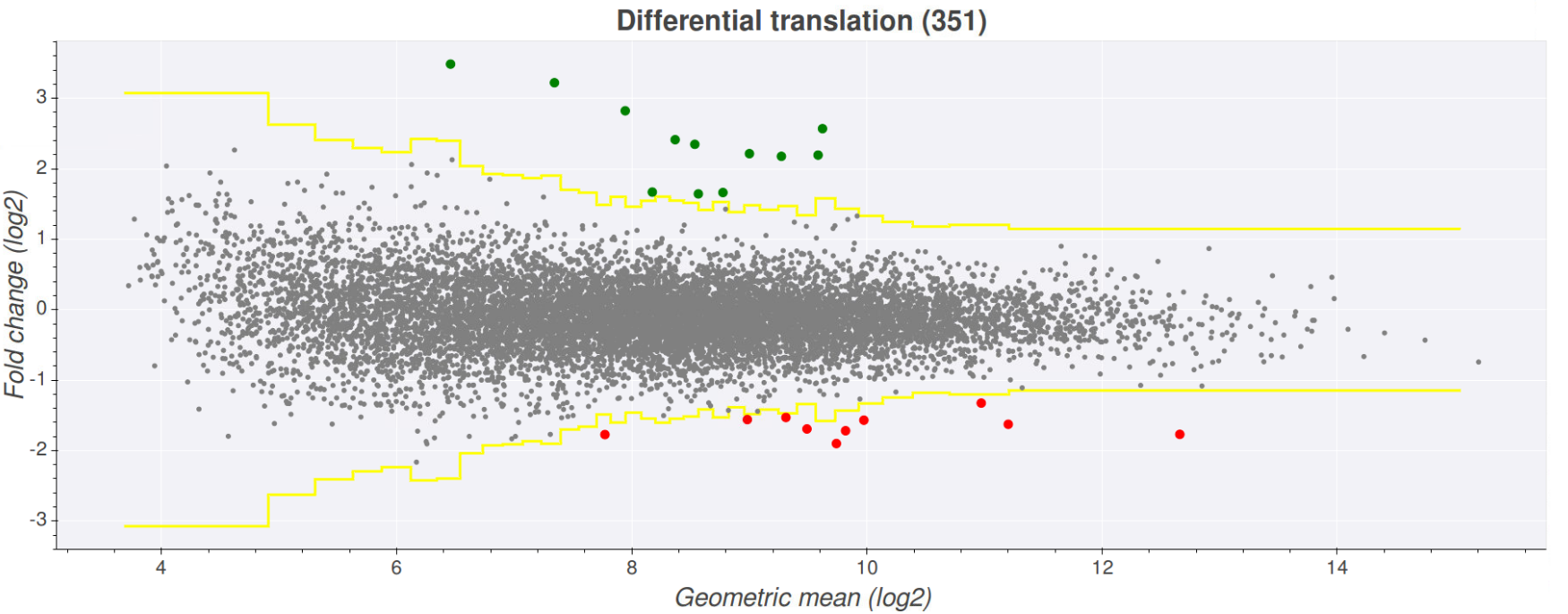
Once you've selected your desired files press the view plot button at the bottom of the page. This will create a plot where the fold-change of the files is represented on the
y-axis and the expression (here expression is determined by the geometric mean of the counts in all files) on the x-axis. The yellow lines on the graph indicate wether the fold
change is above or below the chosen z-score. Transcripts that fall above the upper yellow line are above the z-score and are coloured green (upregulated), while transcripts that
fall below the lower yellow line are below the z-score*(-1) and are coloured red (downregulated). Clicking on any one of the points will open a seperate tab showing the comparison
plot for that transcript with the conditions coloured green/red.
Note: In human and mouse only one principal isoform is used for each gene as determined by appris.
In order to see which transcript is associated with a given point on the plot just hover over the point. This will show a pop up with information such as transcript, gene,
minimum expression and fold change. Clicking on one of these points will open another tab showing the comparison plot page on Trips-viz, which shows the plot for the transcript
you clicked and the files contributing to the plot colour coded red/green.
Plot type
Choose the method used for identifying differentially expressed/translated genes. If correlation is selected only fold changes of transcripts will be displayed with no attempt to identify significant genes. Significantly differentially expressed/translated genes can be found using the z-score approach, DESeq2 or Anota2seq. If DEseq2 or Anota2seq is used a link above the plot allows you to download the inputs/outputs of the relevant software.
Gene type
Carry out the search using coding transcripts (default), non-coding transcripts or all transcripts. If this is not set to coding then region has to be set to "all".
Minimum Z-score/Max p-adj
If using the z-score plot this option allows you to set the minimum Z-score required before a transcript is considered significantly up/downregulated. Z-score represents the number of standard deviations a particular transcript is from the mean. So for example given a minimum z-score of 4, only transcripts 4 standard deviations above or below the mean would be considered significantly up/down regulated. If using the DESeq2 or Anota2seq plot types this values represents the max p-adjusted value that will be used to consider genes significant. The values is a percentage so entering 5 in this box will count all genes with a p-adjusted values below 5% as significant. The default value for the DESeq2 plot is 5 while for Anota2seq it is 15.
Region
This determines which region the counts for a particular transcript will be taken from.
Normalize by mapped reads
In some cases you may wish to compare datasets with a very different number of mapped reads. Ticking this box finds the difference between the groups based on the number of unambiguously mapped reads. The counts for one of the groups will then be reduced to mitigate the difference. For example if there is one dataset in condition 1 with 1,000,000 mapped reads and one dataset in condition 2 with 500,000 mapped reads, the count for every transcript in condition 1 would be divided by 2. This is only applicable when not using the DESeq2 or Anota2seq plot types.
Minimum reads
Any transcripts with less than this number of reads in any group will be ignored. If normalisation is used the minimum applies to the normalised value. This is only applicable when not using the DESeq2 or Anota2seq plot types.
Highlight gene list
Enter a comma seperated list of gene names, these will then be highlighted red/green on the z-score plots and black on other plot types.
Transcript list
Enter a comma seperated list of transcript ids, search will then be carried out only on these transcripts.
Transcriptome info plot
Video tutorial
Plot description
The purpose of these plots is to explore any information inherit to the transcriptome annotations, not related to Ribo-Seq/RNA-Seq or other data types, for example transcript lengths or GC content. Many of the plots have multiple inputs for seperate transcript lists allowing for easy comparisons between groups.
Nucleotide compositon (Single transcript)
Used to explore the nucleotide composition of an individual transcript. Enter a transcript ID in the input box and press "View plot", a plot will be displayed showing a sliding window across the entire transcript of individual nucleotide compositions as well as GC content and minimum free energy (MFE). These can be turned on/off using the legend on the top right of the plot.
Nucleotide compositon (Multiple transcripts)
Used to investigate the nucleotide composition of multiple groups of transcripts. Between 1 and 4 lists of transcripts (comma seperated) can be entered in the boxes at the top right. The nucleotide and region that is taken into consideration can also be chosen here, as well as the plot type (scatter or box).
Lengths plot
Used to investigate the lengths of multiple groups of transcripts. Between 1 and 4 lists of transcripts (comma seperated) can be entered in the boxes at the top right. The region that is taken into consideration can also be chosen here, as well as the plot type (scatter or box).
Gene Count
Displays the number of annotated genes and transcripts in a transcriptome. These are broken down further by the number of annotated coding (green) and non-coding (red) genes/transcripts.
Codon Usage plot
Displays the codon counts of coding regions of all principal isoforms if the supplied list is empty, a custom list of transcrips (comma seperated) can also be entered to only get codon counts from those transcripts.
Nucleotide frequency plot
Build a nucleotide frequence plot centered around the TSS (transcription start site), CDS start, CDS stop, or TTS (transcription termination site). A comma seperated list of transcripts needs to be entered.
ORF Table
Generate a table of uORFs or other ORF types with information such as start/stop positions, length and start codon. Results can also be downloaded as a csv file.
Translated ORF detection
Video tutorial
Plot description
Used to detect translated ORFs in various categories, which can be selected at the top left of the page. Several features will be calculated derived from the selected ribosome profiling data. These features are then ranked, individual ranks are then aggregated to create a global rank. A table will be returned showing ORFs ranked from highest to lowest. Each ORF will have a link to view the ORF on the single transcript plot page with the selected ribosome profiling data where the ORF in question will be highlighted. Only the top 1000 ranked ORFs will be shown on the page but all ranked ORFs can be downloaded in csv format by clicking the link above and to the left of the table. If proteomics data is also selected a column in the csv file will indicate the number of peptides that overlap the ORF in question. If all files in a particular study are selected an aggregated file for that study will be used which will speed up the search significantly.
Start Increase
This feature compares the number of reads 5' of the start codon to the number of reads 3' of the start codon, with the assumption that there should be a large increase in reads at the start if the ORF is translated and thus a large difference between these two values. Only inframe reads are considered from the 5 codons before and after the start.
Stop Decrease
This feature compares the number of reads 5' of the stop codon to the number of reads 3' of the stop codon, with the assumption that there should be a large decrease in reads at the stop if the ORF is translated and thus a large difference between these two values. Only inframe reads are considered from the 5 codons before and after the stop.
Coverage
This feature is dependent on the frame difference feature (highest or lowest). If the frame difference feature (highest) is used, this feature counts the number of positions in the ORF where the inframe count is higher than either of the other two frames, if frame difference (lowest) is used it counts the number of positions where the inframe reads are not the lowest of the three frames.
Frame Difference (highest)
Takes the number of inframe reads and substracts the number of out of frame reads (from whichever of the two is highest).
Frame Difference (lowest)
Takes the number of inframe reads and substracts the number of out of frame reads (from whichever of the two is lowest).
CDS overlap
Limit the search to only ORFs that minimally or maximally overlap a CDS region, values entered are between 0 and 1. If for example the min limit is set to 0 and max limit set to 0.5, the only ORFs that are returned will overlap CDS regions by 50% or less. Values will be changed automatically to the suggested values when switching ORF types, for example setting the max limit to 1 (100%) if searching for nested or CDS ORF types.
Length
Limit the search to only ORFs with a length between the min and max limits (in nucleotides).
Transcripts
Search for ORFs only on principal transcripts, all transcripts or a custom list (enter a comma seperated list in the input box).
Start Codons
Search for ORFs begining with either AUG, CUG or GUG codons.